Cloud HPC removes the queue and the capital cost, and replaces them with a different question: how much hardware should you ask for? Doubling the core count rarely halves the run time, and beyond a certain point it only raises the bill. This article explains what limits parallel performance in CFD and how to size a cloud run sensibly.
Strong and weak scaling
Two measures describe how a solver uses more cores.
- Strong scaling keeps the problem fixed and adds cores. Ideally the run time falls in proportion. This is the relevant measure when you want a given mesh solved sooner.
- Weak scaling grows the problem with the core count, keeping the work per core constant. Ideally the run time stays the same. This is the relevant measure when you want a larger mesh in the same time.
Speed-up on N cores is S(N) = T(1) / T(N), and parallel efficiency is S(N) / N.
Amdahl's law
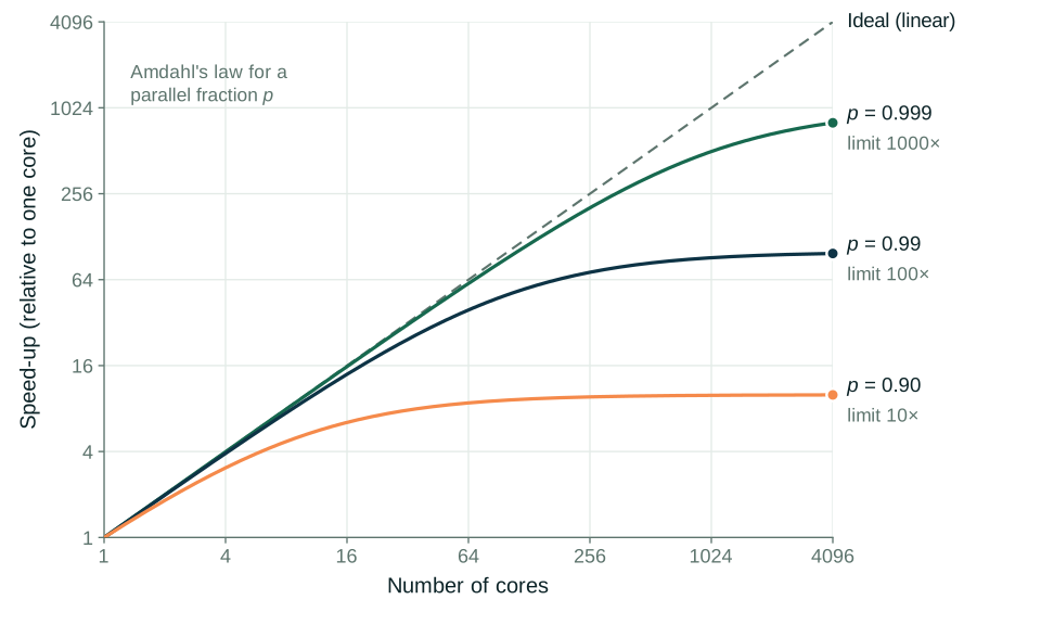
If a fraction p of the work can run in parallel and the rest is serial, the best possible speed-up is
S(N) = 1 / [(1 − p) + p / N]
The ceiling is 1 / (1 − p), however many cores are added. With 99 % of the work parallel, 100 cores give a speed-up of about 50, and the limit is 100. In CFD, communication between partitions adds an overhead that grows with core count, so real curves flatten sooner than Amdahl's law alone suggests.
The cells-per-core rule of thumb
Parallel CFD solvers split the mesh into partitions, one per core, and exchange data across the partition boundaries at every iteration. As partitions shrink, the boundary cells become a larger share of each one and communication starts to dominate the computation.
Parallel efficiency typically falls off below a few tens of thousands of cells per core. The exact figure depends on the solver, the physics and the hardware, so measure it for your own case.
On that basis a 20-million-cell mesh is used efficiently by some hundreds of cores, not thousands. The reliable way to find the number is a short scaling test: run the real case for a fixed, small number of iterations at three or four core counts and compare the time per iteration.

Memory bandwidth and interconnect matter more than core count
Unstructured finite-volume solvers spend most of their time moving data between memory and processor, not on arithmetic. Performance is therefore limited by memory bandwidth. Once the memory channels of a node are saturated, extra cores on that node add little, and running with some cores idle can give nearly the same throughput. This matters most when software is licensed per core.
Across nodes the limit is the interconnect. Partition exchanges are frequent and small, so latency matters as much as bandwidth. Low-latency networking of the InfiniBand or RDMA class lets a job scale across many nodes. Standard virtualised Ethernet generally scales less well, and efficiency can stall after a few nodes. When choosing cloud instances, look for HPC-specific types with high memory bandwidth per core and an RDMA-capable network before comparing headline core counts.
CPU or GPU solvers
GPU-native CFD solvers are now available in several commercial and open-source codes, and for supported physics a small number of GPUs can do the work of a large number of CPU cores. Two constraints apply. GPU memory limits the mesh size per card, and not every model available on CPU has been ported. Check that the full set of physics you need runs on the GPU path before planning around it.
Spot capacity and checkpointing
Spot or pre-emptible instances are spare capacity offered at a discount, on the condition that the provider can reclaim them at short notice. They suit CFD if the run can survive an interruption. That means writing restart files at regular intervals to storage that outlives the instance, and automating the restart. In a multi-node job the loss of any one node stops the run, so the risk grows with node count, and on-demand capacity is often the better choice for long, tightly coupled jobs.
Data transfer and storage
A transient simulation can produce far more data than anyone will examine. Storing it costs money, and downloading it takes time and usually incurs egress charges. Decide before the run what to keep.
- Write full fields only at the intervals the analysis needs, and use surfaces, cut planes and probes for anything sampled frequently.
- Compute time averages and other statistics during the run instead of from stored snapshots.
- Post-process on the cloud side and download images, reduced data and reports.
- Use fast scratch storage during the run, and move what must be retained to cheaper object storage afterwards.
Design sweeps: many small jobs, not one large one
A study of twenty design points is twenty independent simulations. Running them side by side, each at an efficient cells-per-core ratio, gives near-perfect scaling, because the jobs do not communicate with each other. This is where elastic cloud capacity is strongest: the whole sweep can finish in roughly the time of a single case. It also suits spot capacity, since an interrupted case is simply resubmitted. The same applies to the runs of a mesh-refinement study.
National compute in India
Commercial cloud is not the only route. Under the National Supercomputing Mission, run by MeitY and DST and implemented by C-DAC and IISc, PARAM-series systems are hosted at national institutions. The IndiaAI Mission includes a compute pillar that offers GPU capacity to start-ups, researchers and academia. Each programme has its own eligibility and allocation rules, so check them early in planning.
How CFD Pro can help
CFD Pro has HPC tie-ups with Oracle Cloud Infrastructure, IBM Cloud, AWS, Google Cloud and Microsoft Azure, and can connect eligible projects to national compute through the IndiaAI compute programme and the National Supercomputing Mission. To discuss how to size and run your simulation, send us a project brief.